FYI: Continual changes will be made :)
A brief reminder: Check iCal!! All the IW's thus far (#1-4) are due on friday! If you have any questions Mr.O'Brien is happy to assist.
We started class off today by finishing going over the problems from IW #4 and correcting any errors or missing concepts on Anna's scribe post for 9/10 based on this work. Mr. O'Brien noted that the problem he did from the homework last period was not actually number 77, but rather the "OB Version" of 77. We learned that this was due to the fact that in the diagram he drew the bottom point of the smaller triangle should be labeled 'Q'.
We had said that  , but with this new piece of information we now know that the 'P' at the beginning should be a 'Q'! This makes the new inequality read:
  . Note that the book asks for , which we determined would equal
  .
.
The point of all of this was to show that the process used to solve would be the same as shown last class for #77, but the variables used in Mr. O'Brien's would differ slightly from those placed in the book. He then reviewed the steps of the proof,assured that we recognized the function as having origin symmetry, and reminded us that a squeeze creates a situation where the limit of ALL of the functions involved is the same. For a review of the original process of the above problem click here!
The last review item we handled was a warning from Mr. O'Brien about problems such as numbers 33 and 72 listed below:
Q33)
Q72)
Mr. O'Brien commented that the issues students run into on problems like these is simply taking them at face value and thinking they're too easy!
In this case, both involve the limit of  . Both require breaking apart using the limit rules.
Why is the limit  simply one? The only value for 'X' which will not give one is 0/0, which is irrelevant because with limits, we do not care about the value at 0/0, we simply care about the values on either side a.k.a - 0.00001 or 0.00001.
Using this information, we were able to solve the problems accordingly:
A33) ----->  .
.
A72) ----->  .
.
---------------------------------------------------------------------------------------------------------------------------------
*Deep breath* Finished! At this point we moved on to the new work, after a few points to remember:
1) We will be moving onto derivatives next!
2) The homework is on iCal and is 12 problems long. (You can also find it here.)
3) Note that we've been working on page 66 up to this point! This is all very basic, but very important stuff! If you don't fully understand anything we've done so far, ask for help or see any of the following links at the bottom of the 'Questions for the Class' page in the blog, or go to this helpful website for interactive practice problems: http://curvebank.calstatela.edu/limit/limit.htm.
----------------------------------------------------------------------------------------------------------------------------------------------
We took a quick break to fill in the google doc info sheet for Mr. O'Brien before starting to tackle today's goal.
Objective:
- Infinite limits!! (for an introduction style example, see my favorite online help source Patrick!)
The object of today's warm up was to refrain from using technology and attempt to solve limit problems, with and without infinity, by hand by sketching a graph and using it to answer the conditions below.
Warm Up:
a) Sketch (showing all relevant features)
b)  c)
c) 
d)  e)
e) 
After giving us about 10 minutes to attempt the warm up with our partners, Mr. O'Brien graphed the equation on GeoGebra as follows to prove why having the skill set to do these types of limit problems by hand is important:
Upon inspecting the graph versus the function, we noticed that the function should have a gap at the point (-1,2/3), but Mr. O'Brien shows us that one is not visible on the image. Likewise, if you tell GeoGebra to plot the point (-1,2/3), it will without error. (See free object A in blue below)
While you can get it to tell you that there is no value, a.k.a the function is undefined at that point by plugging in f(-1) (See dependent object above) rather than (-1,2/3), if you were not able to tell that there should be a gap, or that you would have to input just the 'X' value into the function to get the program to tell you there is this undefined value, you would be in trouble! This example illustrated a situation in which graphing by hand and solving by using the graph, or by algebra would be more useful. When graphing by hand you ensure the graph give you all the information needed.
Side Note: Wolfram Alpha will graph and give you the limit, and answer to the limit. Will posed the following question though: Can Wolfram Alpha answer limit problems involving infinity? Answer: YES! Proof:
How cool is that! Unfortunately, it was back to the old school method to cover how to solve by hand.
Too make it easier, here is the function in question again:
We determined that the function from the warm up has a few simple relevant features:
1)Asymptotes: -2,2
2)Domain: All Real Numbers EXCEPT -2,2,-1
3)Range: All Real Numbers
If finding any of the above, or the hole in a function tends to trip you up, review these skills using the following site.
Next, we decided we were ready to solve part (b) of the problem since it appeared to be doable algebraically. We began by factoring both the numerator and denominator of the function, in hopes of giving us a new function in which -1 is defined:
Expansion: 
Simplification:
Cross Canceling:  .
.
If we labeled this new function g(x), we found that evaluating for g(-1) gave us -2/-3=2/3 as the answer to (b)! (Note For Future scribes: parenthesis in the denominator of the fraction should be one set around the whole set of numbers, not multiple sets. See change to "expansion" line for proper formatting.)
For parts (c), (d), and (e) Mr. O'Brien wanted us to utilize the sketches we made, so we went over what should go into making a good one. We determined that for this function, a good sketch would note that the function is undefined or has a gap at (-1,2/3), has two asymptotes, one at 2 and one at -2, and has zeros that can be solved for using simple algebra. (the zero we found to be (1,0). We were reminded that having the y-intercept was also useful, and that to find that is x--> 0 we could always substitute that in for all of the 'X's' to get it. This gave us (0,1/4). From these points you can sketch the center part of the function by connecting the dots(here was mine):
The only thing Mr. O'Brien made sure to add about the asymptotes, or the other two pieces of the function effected by them, is that you must ensure they are not volcanic asymptotes which occur where there is a double zero in the denominator of the function. We determined this was not the case in our function however, since to get a double zero we would have to see the following function instead:
 ---->
---->  .
.
Due to this, we were able to assume the regularly shaped ones could be drawn and our graph was complete. We then solved parts (c) and (d) without much difficulty.
(c) At the graph shows no value being approached from either the right or left side of the limit, thus we determined the answer to this part was D.N.E.
(d) At the graph shows that tracing form the left side of the function leads off endlessly. We would generally call this another D.N.E, however we learned a new concept that helps us correctly label this answer from Mr. O'Brien:
When a value is leading off infinitely in different directions, like in part (c) when  , we say that the limit does not exist because there will never be a value reached on either side of the limit to record. When you are coming from only one side with the limit however, like in (d)
  where you come from the left or if d were
  and you were coming from the right, although the limit still will not exist and will be going off into infinity (as proven by the answer to part (c)), we can still say that the limit is approaching either negative of positive infinity. In this case, the limit is infinite and technically doesn't exist, however because we can define it as approaching either negative or positive infinity, we will.
With this information, we determined the final answer to part (d) to be D.N.E;  .
.
Part (e) really represented the new concept of the day. The evaluation of the function at , means imagining what the function would look like when you inputed larger and larger values as they approached infinity. We decided that the larger the value of 'X', the closer the function would get to 0.
*Done!*
An interesting thing to note: either the limit can have the infinity part like this:  , or the answer to the limit problem can be
  .
.
----------------------------------------------------------------------------------------------------------------------------------------------
Now that we had had the bulk of the lesson, we tackled a few practice problems:
Ex/ 
Ex/ 
Ex/ 
Ex/ 
Our guesses were all over the place!
For the first two Mr. O'Brien steered our minds towards a parent function of use, which in this case was f(x)= 1/x. We talked about the fact that the only difference between that and the function in the first two examples was a few shifts. This allowed us to realize, through visualizing the parent graph and shifted graph that the answers did not exist (we still expressed them as -/+ infinity though). Here is what this would have looked like on GeoGebra:
The second two problems posed more of a challenge, and we decided it best to try tacking them numerically. At this point we were introduced to the concept of an end behavior model. Mr. O'Brien explained an end behavior model by using the first equation as an example. He pointed out that as 'X' got infinitlily large, 4x+1 would begin to look a lot like a 4x line graphically, with the same occurance on the bottom with 7x+5 looking more and more like 7x as values increased toward infinity. So, as a whole as 'X' approaches infinity and our theoretical graph gets farther and farther zoomed out, we can say that:
is moving towards being about equal to  .
.
The equation on the left of the equal sign above before simplification would be the end behavior model for this function. This means the horizontal asymptote is also 4/7, which tells us that the answer to the third practice problem is 4/7 as well.
Using the same method of end models, we determined the end model for the last practice problem would look and simplify as follows:
 .
.
If we're looking at the limit of X as the values get smaller and smaller(due to the negative), we know that would be approached.
Finally, Mr. OB referred us to pg. 71 in our books back to the yellow box with notes on the limit rules, which still apply to infinite limit problems, and to an explanation of why the squeeze theorem still works as well. He also pointed out on pg. 72 an interesting exploration problem in a blue box that reminds us that both the numerator and denominator of the function must have existent limits, or else we cannot apply the limit rules that allow us to break them down as they both move towards infinity because you will get 0/0. The following three problems in the box that we did continued to allude to the main point of the exploration: you must know when the limit exists and, if it doesn't, if you can manipulate the function into something that does exist when the function approaches infinite limits. This means that if you find the numerator and denominator to have existent limits, but an undefined value when you plug things in, you may break apart the function using the multiplication or addition rules and the take the simplified form and solve from there.
HW: Finish IW #1-4 for friday. Tonight pg. 76 #3,7,15,27,35-38,53,55,59,61.
P.S. The next scribe will be...SARAH!
P.P.S Update Below!!!
In this lab period we made corrections to this post and then went on the answer homework questions. The few we covered were 36,55,,and 7c. Here is the work for 36&55 and then 7c:
Two important questions stemming from this were: Can you touch the asymptotes in these problems? YES it is a limit for the formation the the graph, not one of your answers on a homework problem for example. and Can you have more than one horizontal asymptote? You can have more than one horizontal asymptote based on the definition in the book:  .
.
Here is a great site to help you practice infinite limits!
http://17calculus.com/calc02-infinite-limits.php


 . In that case of this one, the base is the main variable, and when you sum it all up, the volume is the same as the definite integral.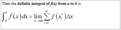
 is simply the chosen point.


 is partitioned into n subintervals of length
  . Let
. Let dennote the midpoint of the
  subinterval. (note the correction from the wording from the picture with actual equations below)
 ? Yes!!


 ) and solve as follows:
 .
.


