Integration by Partial Fractions

Integration by partial fractions can be difficult - it's a good thing we're here to help. Let James and Alex guide you through the tricky world of partial fraction decomposition as it pertains to integrals.

We begin with a difficult example of a function to integrate: let's say you wanted to find something like:

Looks time-consuming, no? Well, there is a way to more easily reduce integrals via the magic principle of decomposition! Decomposition of a fraction is the process of breaking down more complex equations into their component parts. The first thing you should know is that this method of integration is based off an old algebra trick, simply applied to calculus. We all know the Fundamental Thorem of Algebra which states that all polynomials can be factored into linear, irreducible quadratic and/or complex (containing imaginary components) factors. This means that polynomials will always have roots which are either linear (such as x+4, x-7, or 12x etc) or are irreducible quadratics which when "reduced" are shown to be made themselves of factors which contain imaginary numbers, always in pairs. Let's say we're not getting into imaginary numbers in our integrating, and we are happy with leaving our decomposed polynomials in terms of their basic building blocks - linear and irreducible quadratic factors.

An important note, however, is that this method about to be described only applies to equations being integrated who take the form of a fraction (technically all equations are fractions) but with the caveat that the denominator (bottom) of the fraction must have a higher power of x than the numerator (top). In cases where the function being integrated has a higher degree numerator, simple long division of your  integral will suffice to find your answer. 

Lets look at the denominator of the above integration.

The reducible quadratic shown in the bottom of the fraction being integrated above is factored into its component parts, two linear factors (x+3) and (x-2). This is nothing new - we've been factoring polynomials for a long time now. Our new integral looks like this: 

This is the first of the four major cases which apply to integration by partial fractions - the decomposition (breaking down into factors for easier integration) of Distinct Linear Factors (when the fraction denominator being decomposed breaks down into simple linear factors). 

1. Take a look at the following equation and see if you can follow the logic involved.

Why have these constants A and B suddenly been introduced to this process? For the equation in question, it is necessary for some value of A and B to exist so as to make the equality above an accurate statement, right? Some A must exist and some B as well which make this a true statement since the denominators of the two parts of the second side of the equality are factors of the first. We'll demonstrate with a very simplified version of this rule:

If we suppose, this makes sense right? We know that.

If we multiply both sides by a funny form of one, we can create a common denominator to match the one we factored apart. When we do this we can see that the above equation is true. 

Lets apply this simple rule to our more complex function being integrated. We'll use the same multiplication by one strategy to create a common denominator, and use that to create a more simple form of our function so as to integrate without as many problems - we'll be decomposing it. 

 ...all dx, of course.

So how does this help us? Well, now both sides of our equation share the same denominator - let's take it right out. Also, lets drop the integration brackets. They're obscuring our goal right now - to find the values for those two constants A and B and create a more simple equation in order to integrate.

Now, we made a fairly large leap of faith in beginning this problem - mostly, that this equation we're using is differentiable. If we continue to hold this to be true, we assume that this equation we have just found is an identity, meaning that it is true for all values of x in order to be a continuous function which can be integrated at all points. 

If we can plug in any x value and be given a correct result in this equation, we can use this to our advantage! Lets cheat the system! The following is a means of performing fractional decomposition which does not work in every circumstance - its a trick like the "drop the power" rule for differentiation, as it only works in simple cases like Case 1 - Distinct Linear Factors. Lets plug in x values which will result in answers for A and B. Try plugging in x=2

Thus, we know now that B = 2/5

Lets do the same strategy for A: say that x = -3

Likewise, we now know that A = 3/5

Now, lets use this knowledge to decompose our origional integral!

 and thus, plugging in our values, 

This is actually , as the now defined A and B are constants.

The new form of the original integral we've found is much easier to integrate now. By using the rule of the integral of 1/x, and remembering that this integral does not have set limits and thus requires a +C, we find the answer to be:

From that messy fraction integral, we have produced an answer! Nice job!

This trick of setting things equal to zero by exploiting the identity of the function we are using can also be applied to problems which belong to Case 2: repeated linear factors. When you see functions which you need to integrate which contain linear functions as the factors of their denominator, but which are repeated more than once, you approach the problem in much the same way. 

How would you go about attacking this? 

Use the same approach as before, making sure to take into account all possible factors of the denominator. This denominator has many more factors than our original easy example - let's see if we can't find them all.

The parts which go into this function's denominator are (x+1) and (x), yes, but don't forget that its also true that a root for this function is (x+1)^2 and (x+1)^3 as well. With this knowledge, we can set up our decomposed series of fractions. Again, we drop the integral sign for the sake of clarity, and will pick it back up later when we actually solve the integral.

Are you seeing a pattern so far? The fractions we use are comprised of the factors of the bottom of the original function, with letter placeholders over each one which represent constants we will solve for. Integration by partial fractions is a long and painstaking process, but its most important feature is that it yields results. You can probably see how we would go about answering this problem: multiplying by forms of one in order to create one single denominator, then substituting in values of x to isolate constants and solve. Then, we plug in values and perform integration just like the first time. 

Now, lets look at the other two cases which are possible in this method. So far, we've been dealing with distinct linear factors, but Case 3 - Distinct Quadratic Factors and Case 4 - Repeated Quadratic Factors are more difficult to solve as they are often at least semi-immune to this trick we've learned so far. So, let's learn the one true (yet painfully slow) method of reducing these equations down. It starts a lot like all the other forms of decomposition, by breaking down the denominator into fractions bearing the parts of said denominator. In Case 3, we see equations like 

Notice first off that the denominator is made of irreducible quadratics, aka quadratics which can't break down into linear functions without involving the use of imaginary numbers. Thus, they must remain in the form they are in. Why, you may ask, have the simple constants of A and B become so complicated in this new form, with x's and all? When broken apart in this manner, these equations containing quadratic factors must contain generic linear factors with generic terms like A and B and C and D on top instead of even simpler constants, since these denominators must be one degree greater in power than the numerator which they are underneath. When we were only dealing with linear factors, our numerators were one power less than them, having x's raised to the 0 instead of to the 1. Now, we've raised all the powers by one. Case 4 takes this idea to yet another level in much the same relation that case 1 had to case 2. A sample case 4 problem would look like this: 

Just like in case 2, we approach this problem by finding all possible factors and creating a decomposition which reflects them.

Now, this is much more complicated a setup than we've had to deal with so far. Let's learn the principle which will serve us better for these more complicated quadratic decompositions. Our trick works well for easier equations, but there is a longer and more time-consuming method which will work every time. 

We'll use an easy example: let's refer to our original original equation way back in case 1 which told us that the following relationship was valid.  

We will now put a name to this new process - it's called Equating Coefficients. First, we multiply our A's and B's in. 

Now, let's look at the invisible exponents in front of our x.

This is where the equating of the coefficients comes into play: since these two identities are equal to each other, the coefficients of each x^1 should equal out, as well as the coefficients of the x^0. This way, we know that 1 = A+B, and that 0 = 2A+B

We now have two true equations, which can be solved any number of ways - the chief two being either equating of equations, or substitution. We'll demonstrate both.

     1 = A+B                                                 1-A = B

-    0 = 2A+B                                               0 = 2A + (1-A)

____________

     1 = -A

A=-1, substitute back in to find B = 2

Are these answers familiar? They should be, they're the exact same answers we found for this example when we did it via our little trick! Equating coefficients is longer and more time-consuming, but will never fail you. Combine it with the trick (for finding of easily-identified coefficients) in order to get to the values you're looking for, and decompose your function into a more easily-integrated form. If you want any practice, UC Davis has 10 problems which they explain well, which will help you practice the basics.

Scribe post 11/16

Well, what an eventful class! We began with the follow-up quiz, bringing to bear our awesome math knowledge and generally outstanding ability to power through several questions based on the Finely Crafted Opportunity Day™. Everyone was energized and dare I say excited to have such a wonderful opportunity to show off our math knowledge like the proverbial peacock. I'm pretty sure that there was loud jubilation and cries of happiness when the test was handed out, and I think several people even jumped up and thanked OB profusely, begging him for another test to take after the first one was done. Sadly, we were limited to only 40 minutes or so of quiz-related bliss before it was back to the grindstone... of, uh, happiness and wonder. The most enjoyable math grindstone...of fun...yeah.

Even as your faithful scribe was scribbling the last few finishing strokes on his quiz, OB was up front with that special gleam in his eye - you know the one. No, not that one. Yeah, that one. The gleam of intrigue, the one that says we were going to learn something new that day - joy oh joy! I hastened quickly to my seat so as to not miss a second of class time. 

We began with a little light math-related humor: 

What is the significance of this equation, you wonder? Why is the limit necessarily six?

Well, let's do some high-level computation. If you cancel the n on the bottom of the fraction with the n on top, the answer obviously becomes . It's so simple! Math really is easy!

When OB cracked this joke, there was an uproar the likes of which have never been heard in the halls of CHRHS before, and likely never will again. All were doubled over in laughter, many struck to the floor, unable to move from the sheer force of the heaving guffaws they produced. There was so much knee-slapping and raucous chortling that the door cracked in five places and several of the support beams in the school's framework vibrated out of place, causing what I suspect to be irreparable damage to the structure. The windows were blown out with the sheer force of the noise, and the lights overhead all exploded in a rain of glass and sparks from the force of the air expelled by a class laughing uproariously in unison. 

 When the fire department had come and gone and a tarp was put over the gaping window holes, we moved onto another warm up problem:

As we collectively bowed our heads and furiously cogitated over the answer, Duncan beat out Cole by fractions of a second and presented the answer . Could this be true? Let's backtrack - if we take the derivative of this function by multiplying by the power of the cubed x and dropping it by one, we get . Success! Does the function go through (2,4)? , it checks out! Once again, Duncan amazed us all with his math expertise. 

Next, OB moved smoothly into an examination of the antiderivative. What is the antiderivative, you say? Try this link! It's from MIT, so you know it's good!

The example we saw in the above picture is a perfect example of an antiderivative problem - a problem involving finding a function by going backwards from its derivative. 

The antiderivative, it should be noted, is not unique until a condition is put on it. In the above problem, the condition of passing through (2,4) was necessary, otherwise there would be a huge set of functions which are the antiderivative of the derivative shown above. In order to answer the above problem and be just as amazingly well-versed as Duncan, simply look at the problem in the sense of "what would we need to do in order to create a derivative with a squared x in it?" We know how to drop multiply and drop powers in order to find a derivative - what function must we be dealing with then? It has to have  in it, so that when the power is multiplied in front and dropped, we wind up with an x squared. 

From here, we just plug in our (2,4) point and find... wait.... But that's not right! There must be something added to this equation we're finding; something that, when derived, drops out. Something like a constant - lets call it c. . Now this is looking better! What, when added to , makes 4? Why,  of course! It seems we found our c! From there, its as simple as putting together the parts and coming up with Duncan's . Wasn't that a blast? A gas? A lark? Well, it was something.

Just to beat the idea into the ground, here's a few more examples. Let's say we have . What is our f(x)? Working backwards, we antiderive (fancy word) that, in order to get sin(x) as a derivative, we must have started with . It only makes sense - since the derivative of cos(x) = -sin(x), this function would give us the desired derivative. But let's step up the math. Take a look at this example:

How did we know that  ? Lets remember our definition of the derivative of inverse tan that we all obviously remembered perfectly on the followup! 

We know that we may well have a constant c which dropped out of the equation when it was derived, as the example before this one showed us. Thus, we are able to find a function to fit our derivative through the wonders of the antiderivative! Now let's do it again!

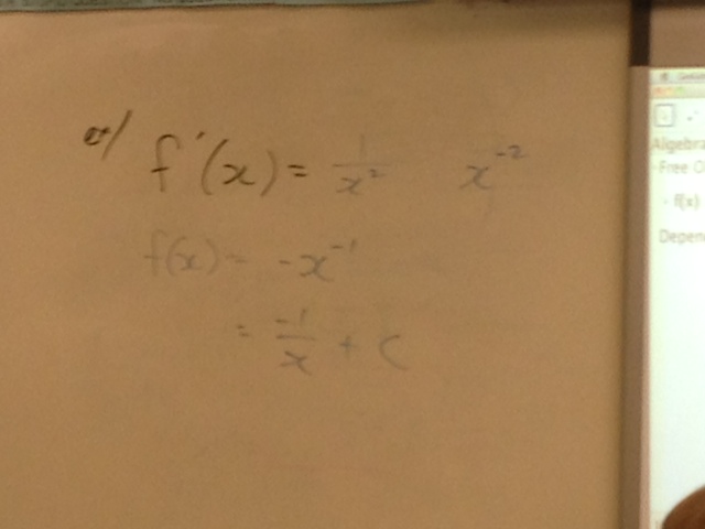
Do you follow what the example does? We know that when x is on the bottom of a fraction, that it can be written as being raised to a negative exponent. In this case, . Using the knowledge Duncan showed so excellently in our first example, lets examine what our function should look like! To get a final value of , we will need a function which, when its exponent is multiplied out in front and then dropped by one, will end up as our desired derivative.  fits well! Dropping down a negative one will make the derivative positive, and the power will descend to -2! But we know that a negative powers moves our x to the bottom of the fraction, leaving the -1 on top. Don't forget that there might be a constant c! 

Confused? So was I! But then OB in his magnanimity decided to show the problem from another angle so that we might truly master its finer qualities. Let's use the natural log to get the same answer - just from a different angle!

We know that the derivative of  is . In this case, the thing on the bottom of the fraction is an . Thus, we know that it must be what was initially natural log'd. Don't forget that constant c! Work backwards from the f(x) we found above if you're still confused - you'll see that taking its derivative works out. Oh wait... does it? When you bring the power out front, that function becomes . Its derivative wouldn't be what we're looking for, it would be , not  like we wanted! Oh woe and sadness, whatever will we do? We could try dividing by 2...

No, that doesn't work. What if we squared it?

Well isn't that an interesting idea... What would that give us? It seems we would need the product and chain rules to fix this mess! This means . Thus, using the product rule we know that . However, this is as far as we can go. There is only one antiderivative that can be found per equation, they are unique. MIT to the rescue again!

Person 1: What's the integral of ¹/_cabin with respect to cabin?

Person 2: A log cabin.

Person 1: No, a houseboat; you forgot to add the C!

*******************************************************************************

We have light homework tonight - IW 3 consists of only 8 problems! However, we do have a quiz next class covering IW's 1, 2 and 3, so if you haven't done 1 and 2 yet, get on them!

To wrap up class, we began an explanation of the Mean Value Theorem which we will have to finish for homework. This theorem, like this intermediate value theorem and extreme value theorem will be useful for reasons to be explained in the examination sheet we have for homework. While at the moment we aren't linking derivatives and integrals, we will be doing so in the future. When we get there, this theorem will be invaluable. 

Let's look at the mean value theorem from a simplified perspective - say you're driving to Augusta from Camden, and you want to average a speed of 50mph for some reason only known to math problem creators. On the trip, at some point your instantaneous rate of speed must hit 50 mph. You may travel half the trip at 1 mph, but in the middle of your ride your speed must increase at an infinitely quick rate so that you can cover the other half at 99. Even when you jump from 1 to 99, your speed passes through 50mph at some point in time. If you're doing a more modest 40mph for half the trip, you must speed up so that your speedometer passes through 50 to reach 60 for the second half of the trip to average out at 50mph. 

Applied to a more abstract mathematical format, somewhere on the interval being looked at there will be a point c where the slope of the secant line of the function between two points and the tangent at said point c are equal. Confusing, right? Lets look at an example like the one on the exploration. 

Here we see the secant line in red connecting the two endpoints of the segment we are studying - call it [a,b] - and the tan line in blue which is parallel to the secant when taken at some point c. OB seems interested - but why is that? As always, Wikipedia has all the answers to life. But why is this so? The exploration will show us.

Doesn't this remind you of something? Something that starts with an I? Something that starts with an Intermediate? Something that sounds like... shmitermediate shmalue shmeorem? Thats right! It does look like the Intermediate Value Theorem! You're so smart! 

Looking at example 1 on the exploration quickly, we notice that there is indeed a point on the interval examined with has a tangent parallel to the secant line drawn between the two endpoints. It seems like the mean value theorem may well hold up. What does Gabe's head have to say about question 2?

Yes Gabe, I agree! It is interesting that its possible for there to be more than one point on a function which has a tangent parallel to a secant drawn between two endpoints of a section.

Alright everyone, make sure that you have the IW's finished tonight as well as the Mean Value Theorem sheet; rest up for the quiz tomorrow also, and don't let those mean values get you down.