Today we began class with a quiz covering IW's 1-4. Then Mr. O'Brien reminded us that the deadline to register for AP Tests is this Friday, but since there's no school on Friday, your best bet is to have the paperwork handed in on Thursday. Next we looked at a video by ViHart about a mysterious number called Wau. She talked about all of wau's properties which were numerous. There was a bit of confusion in the room until we realized wau was just 1. Then O'B spoke some pretty powerful words: "We're done. We've finished calculus." Well, we've almost finished calculus. This led O'B into a discussion about the weeks between now and the AP Test. All of this info can be found on the iCal, but I'll summarize: - O'B is leaving and will not be here next week. IW 6 and 7 will be assigned while he is away. They are a set of FRQ's with answers. Make sure you actually do the FRQ's because there will be a quiz the Friday (March 22) he gets back on IW 5 and the FRQ's. There will be NO number changes, which means we can't use notes. - If you have questions about IW 6 or 7, just post them up and O'B will get to them as soon as he can. We will have 3 hours of in class time to get these done. Thats double the amount of time we need. -March 26 (tuesday): We have a test. IW's 5-8 are due. -March 29 (friday): Supercorrections are due. - April 3: The first grade of Q4 will be the follow up test! - Aril 5: The first quiz of Q4 will be trig values. This is not timed and is re-takable up to 100% -April 9 and 11: Quizzes on FRQ's. NO number changes. Do IW and you'll be set. Closed notes. -April Break: Optional FRQ's - April 24 and 26: Multiple choice section of full AP practice test -April 30 and May 2: FRQ section of full AP practice test -May 6: Supercorrections due for the above test -Tuesday May 7: Deadline for all late work. -Wednesday May 8: AP TEST - No work will be accepted after the AP test. It's a waste of everyone's time. We will then do a project as our final exam and we are allowed to work in partners or threesomes. Now on to IW 5. Although the link for this IW can be found on the ical, make sure you write all the answers out in your notebook, not just on the handout. IW#5 Question 31: Find the volume of the solid generated by revolving the region bounded by the parabola y=x^2 and the line y=1 about (a) the line y=1 (b) the line y=2 (c) the line y=-1 Here is a graph of this scenario courtesy of Connor Lane:
A) So, in part a, we are revolving this around the line of y=1 which happens to be one of the boundaries of the shaded region. This means that when we rotate it, it's radius will just be the distance between the line y=1 and the curve y=x^2. So, this gives us:
Notice that the limit is just from 0 to 1. Even though the shaded region goes from -1 to 1, we compensate by doubling the integral since it is symmetric about the y axis. B) Okay, so now we're rotating it about the line y=1. When we take a cross section of this, it is going to give us a washer. This means we need to subtract the inner circle from the outer circle to get the area of the washer, then multiply it by that small thickness, dx.
The first term of the integrant is the big radius, while the second is the small radius, which then become the big circle and the small circle, respectively when you multiply them by pi and square them. Multiple all this by that small width to get the area! C) Now we are rotating it about the line y=-1. In part B, the outside of the solid had a curve to it, while the inside was flat. It made a roller blade-esque wheel. However, now the outside radius remains the same, while the inside radius is changing. So, we have to take the big radius that is formed between the line y=1 and y=-1 and subtract the little radius from it. This little radius is changing and is formed between y=x^2 and y=-1
Next we looked at #1 from IW 5 Find the volume of the solid with semicircular cross sections whose base is in the xy-plane between the x-axis and the curve y=sqrt(x) over [0,9]. See the visualization here. Remember that the area of a semi circle is just half of the area of a circle. So, (1/2)πr^2. Here is a graph of what we're looking at:
So, as you can see, the diameter will be changing. And remember, we're interested in the radius so we'll have to split the diameter in two! This gives us:
Today we began class by listening to a very intriguing piece about struggle and its connection to learning. We learned that "struggling is a chance to show that you have what it takes emotionally to overcome the problem, by having the strength to persist through that struggle" and that "academic success is not as much about whether a student is smart, academic success is about whether a student is willing to work and to struggle". As we listened to this, O'B was suggestively flaunting supercorrections as if there was a method to his madness. In case you're looking to get motivated, that piece by NPR can be found here. If that's not enough motivation, check out one of my personal favorites:
"When you want to breathe as bad as you want to succeed, then you'll be successful". "Sleep is those people who are broke. I don't sleep" It is hard work that makes a calculus student successful, and its hard work that makes math teachers smile
Next we talked a bit about supercorrections. If you didn't get them back today, you will get them back tomorrow. Also, prepare for the follow up test on Friday by using this blank copy of the test. Mr. O'B had the following words of wisdom for the following test problems to help us prepare for the follow-up: #1: A derivative is a rate of change in a moment of time. It's the slope of the tangent line at any particular point #2: Make sure you know the relationship between position, velocity, and acceleration #3: If you want differentiability, you must have the same derivative from the left and right #5: Make sure you're substituting in the Y value, not the X value! #6: On the follow-up test, this question might be non-multiple choice. That means you can leave the answer in an form you'd like. For the calculator side, don't forget about nDeriv and solver! #7: Make sure you know derivatives of logs and inverse trig functions for the follow up #8: Make sure you're comfortable with the limit definitions #9: Sometimes you'll have to use the product rule in conjunction with the chain rule! Also know your log properties. They can be found here #11: Know the derivatives of exponential functions. #12: The follow up may ask a similar question but with inverse tangent or inverse cosecant #13: The derivative finds you a slope of the tangent line at ANY point. You have to plug in the value of x to find the slope at a specific point. #14: This is just simply asking for the derivative of cotangent evaluated at π/4 #15: Remember that with a limit definition, the slope of the tangent line on the top of the fraction divided by the slope of the tangent line on the bottom of the fraction will give you the limit value.
Mr. O'B then proceeded to tell us that the questions on the follow-up test will be completely random. He likened his method of choosing which questions to pick to the method by which George Bush's speeches are put together, as seen in this video: (skip to 1:24)
Now we got down to business.
Our objective for today: Learn about absolute (global) extrema and relative (local) extrema.
To begin, we looked at the convoluted and confusing definition of absolute extrema values
So, what this definition is basically saying is that the absolute max is the largest y value for a function, and the absolute min is the smallest y value for a function.
Let's put this into action by looking at the following functions on the following domains:
a)all reals
b) [0,2]
c) (0,2]
d) (0,2)
First let's look at the function with the domain of all reals:
So, this function has no absolute maximum, because it just keeps on going! However, it does have an absolute minimum. The absolute minimum is 0 when x=0. Now let's look on the interval of [0,2]:
This has the same absolute minimum of 0 when x=0, but now there is a absolute maximum! Here the absolute maximum is 4 when x=2. Now let's look at the interval of (0,2]:
Okay, so here again we have an absolute maximum of 4 when x=2. However, now that 0 isn't defined in our function, what is the smallest y value? What is the absolute minimum? Maybe it's .001? Or .00001? No no. You could go on and on, but there is always a smaller number you could stick in there, so there is actually NO absolute minimum for this function. Now let's look at the interval of (0,2):
The same concept as we just discussed applies here. Since neither 0 nor 2 is defined in this function, what is the largest y value, and what is the smallest y value here? What are the absolute extrema's? Well in this case, there aren't actually any! When a function like this is on a completely open interval, there wont be any absolute extrema. This brings us to the extreme value theorem which states that if a function is continuous on a closed interval [a,b], it will have an absolute max and an absolute min. Check out this applet that looks at the theorem. Look at these three graphs–they all are on the closed interval [a,b] and they all have global maximum and global minimum values:
Now it's time to look at relative extrema! To do this first, we looked at the definition on page 193. It is even more convoluted and confusing than the first definition we looked at! Hip hip hooray! Here it is:
So what this is basically saying is that if you look on a little open interval of a function, and you have a point that is the highest, or a point that is the lowest, you have local extrema! Following that logic, we can assert that if you look at all of the local extrema, you will find the global extrema as well! To get a more visual representation of this, we took a look at the figure on the same page:
So, as we can see here, this graph has local minimums, local maximums, absolute maximums, and absolute minimums. So, for example, if we're looking at the open interval of (a,e), the local maximum is indicated where x=c. Notice anything about these local extrema? They occur in three places: where the derivative of the function is 0, where the derivative of the function is undefined, and at end points. Where f'(x) is equal to 0 or undefined are known as critical points. So, we can say that extrema only occur at critical points and end points. The derivative of the function is equal to 0 where you have a gradual change, such as at x=c. The derivative of the function is undefined at a cusp or corner such as where x=d. Critical points can be broken down even further into stationary points. Stationary points are where f'(x)=0. They are called this because that's where the function goes up, stops, then goes down, or goes up, stops, then keeps going up. One thing to keep in mind is that just because you have critical points, DOESN'T mean you have extrema. Take this functions, for example:
You see, that at x=0, the derivative is equal to zero. Therefore, there is a critical point on this graph. However, this graph has no extrema! There are no values that are the lowest or the highest. To finish up class, we took a look at two examples of the application of our newly found knowledge! The first question asked us to find the extreme values of :
on the closed interval of [-2,3] algebraically, then to confirm graphically. So, here's what we have to do: We know that we'll find extrema where the derivative is 0, or undefined, or at end points. So, we need to solve for where the derivative is equal to zero, or undefined, and the endpoints, which are given to us as -2, and 3. With these values, we then need to plug back in to the original equation to see what values are the biggest or smallest to give us our extrema. Look at the following work below:
So, as you can see, when we find the derivative, it will never be equal to zero, so we must find where it will be undefined (where the denominator is equal to 0), and this occurs when x is zero. When we then plug in the critical points and end points, we can determine which is the smallest, and which is the biggest, which are our local extrema! We can now check this graphically to see if we're right! When we do that, we get the following graph:
Looks like we're spot on!
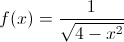
The next problem we looked at was to find the extreme values for the following function using a graphing calculator:
When you plug this into your calculator, it tricks you! It looks like there is both a global max and a global min. However, there is only a global minimum. This is because there are vertical asymptotes. However, the calculator doesn't show this, so it just looks like the function ends. Here is how you tackle this problem algebraically:
To make the derivative undefined, x has to be 2 or -2. To make the derivative zero, x must be 0. When you plug these values back into the original function, 2 and -2 make the function undefined (the vertical asymptote we already discussed), and 0 makes the function 1/2 which becomes our global minimum.
Update:
Thinking about all of these minimum's and maximum's, what does it all mean? Let's take a quick look at the connection between maximum's, minimum's, functions, first derivatives, and second derivatives.
So, think about the function x^2... We know what that looks like: a parabola opening upwards. So, we know that the function has a minimum at the very bottom of the curve. And at the bottom of the curve, the parabola flattens out for a second to give us local linearity, such that the slope at the very bottom is 0. That means that at the origin, when we look at our derivative, it will be zero. But what is the graph of the derivative doing before and after that? Well, let's think about to the left of the parabola. The slope is really really negative, and then as it gets closer and closer to zero it becomes less and less negative and begins to flatten out until it is zero, then to the right of the origin, the slope gets bigger and bigger and more positive. So, the derivative will start negative, pass through the origin (so it is equal to zero) then keep going up. It will be a line! In fact, it will be the line of 2x! Now what about the second derivative? The first derivative has a constant slope, which means that the second derivative will just be a line, the line of y=2 to be more exact! So, a graph with an absolute minimum has a derivative with a positive slope, and a second derivative that is a positive horizontal line. What about a graph with just an absolute maximum? Like -x^2. Think about everything we just talked about in reverse. The derivative will now have a negative slope, and the second derivative will be a negative horizontal line. The graph of -x^2 is known as concave down, and the graph of x^2 is known as concave up. These concavities can tell us a lot about the behavior of the first and second derivatives.