To Be Continued...

The class started with a festive Valentines Day exploration (two to be exact), that you can find right here: https://dl.dropbox.com/u/3243156/CHRHS/apcalc/U4%20Definite%20Integral%20%26%20Trapezoidal%20Rule.pdf
...and looks like this:

We were given approximately 10 minutes (uninterrupted except by an interjection from Becca at the back of the room who was offended when Sarah chose her "eye candy" over her best friend for the task of tackling the exploration) with a partner to try out the problems, the first side dealing with general definite integrals, and the second with the Trapezoidal Rule, which will be mentioned in detail latter in the post and was alluded to in IW #6.
----------------------------------------------------------------------------------------------------------------------------------
Here are a few notes about the Valentines Sheet:
Side #1
First thing's first; know what type of graph your dealing with! In this case it is velocity. Second thing to check is the units and scale, in this case meters/second and seconds. Also, remember D= S * T , or the area underneath the function. This is how you can solve the first question.
1) 1,200
2) estimates between 27-28 squares
3) Each square is = 50ft (Check the scale!)
4) 1,420


OB didn't post answers to these explorations ( :( ), and this one wasn't gone over in as much detail, so solutions can be found on the internet is needed.
We started a discussion about why you would ever use trapezoids instead of rectangles. Being the lazy senioritis infected seniors most of us are (proudly), we gave the simplest possible answer first that seemed like what OB might want to hear: the trapezoids must be easier to work with. **Wth?** We didn't think that one through....the next attempt however was much better, as we decided that the method must be overall more accurate, which it is.
***Trapezoids underestimate for functions that are concave down and overestimate for concave up, however still, more accurate most times than rectangles can be!***
Here is where we started playing with calculating trapezoidal sums on GeoGebra, which will be detailed more later in this scribe post. It was important to note however that the heights always stay the same, the base varies. When you sum them all up, you get your answer.
After all this, we began...
----------------------------------------------------------------------------------------------------------------------------------
Here are a few notes about the Valentines Sheet:
Side #1
First thing's first; know what type of graph your dealing with! In this case it is velocity. Second thing to check is the units and scale, in this case meters/second and seconds. Also, remember D= S * T , or the area underneath the function. This is how you can solve the first question.
1) 1,200
2) estimates between 27-28 squares
3) Each square is = 50ft (Check the scale!)
4) 1,420
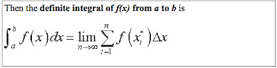
During the discussion about this side of the exploration, Alex W. was on target in explaining
that symbolically the function in definite integral form would look like:

with the 'S' being the integral sign, the first part of the integral (lower one) on the bottom, in this case 0 and the second part (higher one) on the top, in this case the 20. Those two values are called the limits. The other parts of the definite integral form are detailed in the image above.
OB posed an interesting question however (couldn't just let a student get the entirely of a question right without trying to confuse him/her with another part to the question), which was "Why do we need to include the (dt)?" Well, the function needs to take into account B * H . With indefinite integrals (regular integrals) this is unnecessary, but since it is here the (dt) has more meaning because the B * H aspect comes form the elongation because it is a summation of rectangles, a Riemman's sum.
We also looked at the graph towards the end done on the board:

Checking units again, its inches squared times inches. We discussed how a cross sectional cut of a football would look like...a circle? a sliver? and finally arrived at a diamond shape. When calculating cross sectional area of anything, there won't be much to calculate, but Mr. O'Brien pointed out that the more you take of the football, the more the curve goes down and then down some more until the get to the middle, where the cross sections then get smaller, since the football is symmetrical.
If you think about it, its like geometry! Think about finding the volume of a cylinder, you would use the formula  . In that case of this one, the base is the main variable, and when you sum it all up, the volume is the same as the definite integral.
. In that case of this one, the base is the main variable, and when you sum it all up, the volume is the same as the definite integral.
The last note on the first side was that you should ALWAYS TRY TO GET: graph ---> analytical function ---> calculator.
Side #2
OB didn't post answers to these explorations ( :( ), and this one wasn't gone over in as much detail, so solutions can be found on the internet is needed.
We started a discussion about why you would ever use trapezoids instead of rectangles. Being the lazy senioritis infected seniors most of us are (proudly), we gave the simplest possible answer first that seemed like what OB might want to hear: the trapezoids must be easier to work with. **Wth?** We didn't think that one through....the next attempt however was much better, as we decided that the method must be overall more accurate, which it is.
***Trapezoids underestimate for functions that are concave down and overestimate for concave up, however still, more accurate most times than rectangles can be!***
Here is where we started playing with calculating trapezoidal sums on GeoGebra, which will be detailed more later in this scribe post. It was important to note however that the heights always stay the same, the base varies. When you sum them all up, you get your answer.
How do limits tie into all this? The limit is the actual value, which on GeoGebra you can do by typing in the 'integral' command. You can get that, and the trapezoid answer and note the difference in error.
A few last things to note on the end of this back side:
- If it asks you for the fastest ____? Look at the maximum.
- Rate of change =derivative
- This function comes slowly to a stop
After all this, we began...
----------------------------------------------------------------------------------------------------------------------------------
DAILY GOALS:
1) Become more comfortable with Riemann's Sums and Definite Integrals
2) Be able to use resources (calculator and GeoGebra) to solve such problems
3) Get a full grasp on the analytical vs. visual (graphic) interpretations of definite integrals
Let's recap for a second.....
***START REVIEW***
Def-i-nite In-te-gral
(Noun)
***An integral expressed as the difference between the values of the integral at specific upper and lower limits of the independent variable.***
Although that definition is the dictionary's interpretation, it nicely and simply sums up the book's definition and the equation below:
Remember, the function f(x) must be continuous and have an interval divided into n sections (which Mr. O'Brien says don't actually have to all be the same width because either way the values will be approaching 0 as they get smaller and smaller, and as any one of the rectangles approaches the limit the values will converge). Also, the is simply the chosen point.
***END REVIEW***
Next, Mr. O'Brien asked everyone to get out their IW #6 and fire up GeoGebra. The topic of discussion, with five main subtypes was:
Rectangle Approximation Methods (RAM)
Let's recap for a second.....
***START REVIEW***
Def-i-nite In-te-gral
(Noun)
***An integral expressed as the difference between the values of the integral at specific upper and lower limits of the independent variable.***
Although that definition is the dictionary's interpretation, it nicely and simply sums up the book's definition and the equation below:
Remember, the function f(x) must be continuous and have an interval divided into n sections (which Mr. O'Brien says don't actually have to all be the same width because either way the values will be approaching 0 as they get smaller and smaller, and as any one of the rectangles approaches the limit the values will converge). Also, the
is simply the chosen point. - To solve definite integrals on your calculator, refer back to Anna's scribe post.
- To practice some definite integrals and do some Chocolate-Studded Dream Cookie baking, here is a (yummy) activity! (someone should do this and bring these in...or make OB do it...HINT HINT)
***END REVIEW***
Next, Mr. O'Brien asked everyone to get out their IW #6 and fire up GeoGebra. The topic of discussion, with five main subtypes was:
Rectangle Approximation Methods (RAM)
- MRAM (Midpoint Sum): The midpoint method takes the midpoint of a single, normal Riemman's bar and uses it to approximate the height of that bar a MRAM analysis.
- LRAM (Left Hand Sum): Using a left hand sum, the point farthest to the left on each normal Riemman's bar is the determiner of height for the bars.
- RRAM (Right Hand Sum): Using a right hand sum, the point farthest to the right on each normal Riemman's bar is the determiner of height for the bars.
- Upper RAM: uses highest possible rectangle values. These points may be sometimes more left, right, or in the middle of the normal 'Integral' function bars GeoGebra can also generate, depending on where that upper point is.
- Lower RAM: uses lowest possible rectangle values. These points may be sometimes more left, right, or in the middle of the normal 'Integral' function bars GeoGebra can also generate, depending on where that low point is.
There is also the promised trapezoidal sum, which is obviously separate from the above rectangular methods. On GeoGebra, trapezoidal sums can be taken unlike on your calculator, and are found by inputing the following:
TrapezoidalSum[ <Function>, <Number a>, <Number b>, <Number n> ]
We practiced finding the trapezoidal sum graphically on GeoGebra with one of the equations from the exploration. Here is what mine looked like:

The slider function for n allowed us to come to the conclusion that as n gets larger, the integral gets smaller, until finally if you set your slider to a Max of 100 and approach it, the area under the function appears to be almost completely shaded in by the very close bars.
_______________________________________________________________________________
So taking a step back, what is the difference between rectangle and trapezoidal methods?
Well, the first three sums in value are picked to make rectangles, whereas in trapezoids you divide into the number and take a point at beginning and end.
_______________________________________________________________________
For midpoints you take the point in the middle of each interval, and thats the value you use to find the height of the rectangle. (see image below)

The advantage of the midpoint method is that if the function is increasing or decreasing you get some of the area that is missed and added to balance themselves out, lowering overall error.
The sum from the left or right, take points to the left or right of interval as evident in the names. Using left it is important to note that you are overestimating when the function is decreasing or underestimating when it is increasing. Consequently, using the right sum (in right it is the opposite: overestimating when the function is increasing and underestimating when the function is decreasing. Below are, in order from left to right, the images of these sums draw on top of the 'definite integral' function on GeoGebra.


After this, using the methods for inputting (below) into GeoGebra listed in the same order as above, we took time to play around and try to use all of these functions. To see the first three rectangular approximation methods in an interactive way, click here.
- RectangleSum[ <Function>, <Start x-value>, <End x-value>, <Number of rectangles>, <Position>]
- LeftSum[ <Function>, <Start x-value>, <End x-value>, <Number of rectangles>]
- UpperSum[ <Function>, <Number a>, <Number b>, <Number n> ]
- LowerSum[ <Function>, <Number a>, <Number b>, <Number n> ]
While the interactive applet above this shows the first three, Cal skillfully got all five rectangular approximations not only correctly inputed with a slider, but also interactive..take a look!
Murmurs of #PrettyMath went around.
Mr. O'Brien added a last comment that rectangles of error never change in height, only in base (EX: entire 0-10 interval divided by number of rectangles).
Now that we'd visually played with Riemman's Sums, definite integrals, and found the prettier side of math, we moved on to practice problems.
----------------------------------------------------------------------------------------------------------------------------------
EX #1: The interval  is partitioned into n subintervals of length
  . Let
. Let dennote the midpoint of the
  subinterval. (note the correction from the wording from the picture with actual equations below)
is partitioned into n subintervals of length . Letdennote the midpoint of the subinterval. (note the correction from the wording from the picture with actual equations below)
EVALUATE:

The first problem is designed to scare you, Mr. O'Brien explained. “Horribly scary, scarily, scary, AHHHH” says OB to be exact. This is asking for an evaluation of the limit of a sum.... of craziness.
CROSS YOUR FINGERS its a Riemman sum, and you can use the definite integral and your calculator to solve.
But how do you know if its a Riemman sum? If the function, representing the height, and the
representing the base are present and the variables can be substituted out for simpler 'x' s, can you find the interval? In this case, can you find the definite integral on the interval from of  ? Yes!!
The fastest way to solve this now that its been translated from gross math slang to true english is on the calculator using the wonderful (fnInt) button. It would look like this typed in: MATH, fnInt (f(x), -2,1), which yields a final answer of -4.5 , no approximations necessary. All in all, after practicing a few of these and learning to see the real question behind the information given, these types of problems are calculator friendly and should only take a few seconds to complete on the AP exam! As OB says, "DONE".
If you are unlucky enough to get problems, like the final three examples from class today, that are non-calculator so (fnInt) isn't available...well that sucks...therefore, we will deal with those tomorrow.
HOMEWORK: Super Corrections for Quiz #2 (NB: grading will be different than usual, so don't focus on the original work and rather make sure your corrections are thorough and use multiple resources!)
Also, all IWs collected Friday of next week!
**The links from the last IW are now fixed and easily accesible. Answers to the last IW are also now available here.
_________________________________________________________________________________
Class 40 minutes:
VIP: Super Corrections due by 12:00am Friday the 1st!! Below are the new rules!

Make a spreadsheet: times vs. velocity vs. position vs. acceleration in a table.
ALL GRAPHS AND TABLES SHOULD BE PRINTED (not optional)

Annotate it all together; make sure you don't forget to include the steps to getting the answer if you didn't have technology again. Add a SHORT part about what you did in the first 15 minutes.
------------
Class Work

The first thing to ask yourself when dealing with these problems in what do I know? For example, in the first problem you should note that the equation is the equation of a circle in disguise.

BAM, circle. We also know that the definite integral is the area bound by the x-axis (gotten from rectangular sum). Going off these two concepts, we can set y equal to the height portion of the equation (  ) and solve as follows:
) and solve as follows:
Now it is easier to see the circle connection. Therefore, the definite integral of the first problem is  .
.
.
For the second problem, you have to solve without technology (yikes). A good guess would be 1.5, since everything from 2-3 cancels out due to the negative heights, which cannot be had, and the fact that the error from above and below cancel each other out, as discussed above when summing all the areas up:

Even though that was a non-technology problem, we used one to look at the canceling that was occurring, so Anna asked if it was possible to do these without one at all. What if the equation isn't a nice geometric one? Mr. O'Brien said you did, and that, again, fnInt is your best friend. However after solving the third question with this method, he admitted that he LIED and that we did not know how quite yet, but that we will know how to think cleverly, look for a possible graph, and determine how to add up all the area to get the definite integral sin technology in a few classes...oh joy!! ( -__- )
Here is the lie in action on camera, and OB showing how quickly and skillfully his fnInt method works for the third problem:
We finished class by looking at the exploration on page 283 and figuring out the answers as a class. Here's what we came up with, and a brief reason why.
- -2
- 0 (+, - cancel out)
- 1 (symmetry of sine)
- 2+2pi
- 4 (double area)
- 2 (shift over to 2, but go to 2+pi = no change)
- 0 (-a to a cancels)
- 4 (base times two ,length same)
- 0 (+1, -1 cancel)
- 0 (odd function, cancels out)
For a good reference for what may be in our future about how to find the definite integral manually, take a look at this extremely easy to understand video!
The next scribe will be Cole Ellison.


