https://docs.google.com/document/d/1QUP7M0iVjgC6LfziFpt05SrBRivXxsHL3eQTHrg5gcE/edit
Tuesday, November 27, 2012
Thanksgiving Scribe Post
Post in Google Docs:
https://docs.google.com/document/d/1QUP7M0iVjgC6LfziFpt05SrBRivXxsHL3eQTHrg5gcE/edit
https://docs.google.com/document/d/1QUP7M0iVjgC6LfziFpt05SrBRivXxsHL3eQTHrg5gcE/edit
Sunday, November 18, 2012
Scribe post 11/16
Well, what an eventful class! We began with the follow-up quiz, bringing to bear our awesome math knowledge and generally outstanding ability to power through several questions based on the Finely Crafted Opportunity Day™. Everyone was energized and dare I say excited to have such a wonderful opportunity to show off our math knowledge like the proverbial peacock. I'm pretty sure that there was loud jubilation and cries of happiness when the test was handed out, and I think several people even jumped up and thanked OB profusely, begging him for another test to take after the first one was done. Sadly, we were limited to only 40 minutes or so of quiz-related bliss before it was back to the grindstone... of, uh, happiness and wonder. The most enjoyable math grindstone...of fun...yeah.
When the fire department had come and gone and a tarp was put over the gaping window holes, we moved onto another warm up problem:

=x^{2} "This is the rendered form of the equation. You can not edit this directly. Right click will give you the option to save the image, and in most browsers you can drag the image onto your desktop or another program.") Next, OB moved smoothly into an examination of the antiderivative. What is the antiderivative, you say? Try this link! It's from MIT, so you know it's good!
Next, OB moved smoothly into an examination of the antiderivative. What is the antiderivative, you say? Try this link! It's from MIT, so you know it's good!


Person 1: What's the integral of 1/cabin with respect to cabin? Person 2: A log cabin. Person 1: No, a houseboat; you forgot to add the C!
Applied to a more abstract mathematical format, somewhere on the interval being looked at there will be a point c where the slope of the secant line of the function between two points and the tangent at said point c are equal. Confusing, right? Lets look at an example like the one on the exploration.


Even as your faithful scribe was scribbling the last few finishing strokes on his quiz, OB was up front with that special gleam in his eye - you know the one. No, not that one. Yeah, that one. The gleam of intrigue, the one that says we were going to learn something new that day - joy oh joy! I hastened quickly to my seat so as to not miss a second of class time.
We began with a little light math-related humor: }{n}=6 "This is the rendered form of the equation. You can not edit this directly. Right click will give you the option to save the image, and in most browsers you can drag the image onto your desktop or another program.")
What is the significance of this equation, you wonder? Why is the limit necessarily six?
Well, let's do some high-level computation. If you cancel the n on the bottom of the fraction with the n on top, the answer obviously becomes =six "This is the rendered form of the equation. You can not edit this directly. Right click will give you the option to save the image, and in most browsers you can drag the image onto your desktop or another program.") . It's so simple! Math really is easy!
. It's so simple! Math really is easy!
When OB cracked this joke, there was an uproar the likes of which have never been heard in the halls of CHRHS before, and likely never will again. All were doubled over in laughter, many struck to the floor, unable to move from the sheer force of the heaving guffaws they produced. There was so much knee-slapping and raucous chortling that the door cracked in five places and several of the support beams in the school's framework vibrated out of place, causing what I suspect to be irreparable damage to the structure. The windows were blown out with the sheer force of the noise, and the lights overhead all exploded in a rain of glass and sparks from the force of the air expelled by a class laughing uproariously in unison.

As we collectively bowed our heads and furiously cogitated over the answer, Duncan beat out Cole by fractions of a second and presented the answer =\frac{1}{3}x^{3}+\frac{4}{3} "This is the rendered form of the equation. You can not edit this directly. Right click will give you the option to save the image, and in most browsers you can drag the image onto your desktop or another program.") . Could this be true? Let's backtrack - if we take the derivative of this function by multiplying by the power of the cubed x and dropping it by one, we get . Success! Does the function go through (2,4)?
. Could this be true? Let's backtrack - if we take the derivative of this function by multiplying by the power of the cubed x and dropping it by one, we get . Success! Does the function go through (2,4)? +\frac{4}{3} "This is the rendered form of the equation. You can not edit this directly. Right click will give you the option to save the image, and in most browsers you can drag the image onto your desktop or another program.") , it checks out! Once again, Duncan amazed us all with his math expertise.
, it checks out! Once again, Duncan amazed us all with his math expertise.
The example we saw in the above picture is a perfect example of an antiderivative problem - a problem involving finding a function by going backwards from its derivative.
The antiderivative, it should be noted, is not unique until a condition is put on it. In the above problem, the condition of passing through (2,4) was necessary, otherwise there would be a huge set of functions which are the antiderivative of the derivative shown above. In order to answer the above problem and be just as amazingly well-versed as Duncan, simply look at the problem in the sense of "what would we need to do in order to create a derivative with a squared x in it?" We know how to drop multiply and drop powers in order to find a derivative - what function must we be dealing with then? It has to have  in it, so that when the power is multiplied in front and dropped, we wind up with an x squared.
From here, we just plug in our (2,4) point and find... wait... . But that's not right! There must be something added to this equation we're finding; something that, when derived, drops out. Something like a constant - lets call it c.
  . Now this is looking better! What, when added to
  , makes 4? Why,
  of course! It seems we found our c! From there, its as simple as putting together the parts and coming up with Duncan's . Wasn't that a blast? A gas? A lark? Well, it was something.
Just to beat the idea into the ground, here's a few more examples. Let's say we have =sin(x) "This is the rendered form of the equation. You can not edit this directly. Right click will give you the option to save the image, and in most browsers you can drag the image onto your desktop or another program.") . What is our f(x)? Working backwards, we antiderive (fancy word) that, in order to get sin(x) as a derivative, we must have started with
. What is our f(x)? Working backwards, we antiderive (fancy word) that, in order to get sin(x) as a derivative, we must have started with =-cos(x) "This is the rendered form of the equation. You can not edit this directly. Right click will give you the option to save the image, and in most browsers you can drag the image onto your desktop or another program.") . It only makes sense - since the derivative of cos(x) = -sin(x), this function would give us the desired derivative. But let's step up the math. Take a look at this example:
. It only makes sense - since the derivative of cos(x) = -sin(x), this function would give us the desired derivative. But let's step up the math. Take a look at this example:

How did we know that =tan^{-1}(x)+c "This is the rendered form of the equation. You can not edit this directly. Right click will give you the option to save the image, and in most browsers you can drag the image onto your desktop or another program.") ? Lets remember our definition of the derivative of inverse tan that we all obviously remembered perfectly on the followup!
? Lets remember our definition of the derivative of inverse tan that we all obviously remembered perfectly on the followup! =\frac{1}{x^{2}+1} "This is the rendered form of the equation. You can not edit this directly. Right click will give you the option to save the image, and in most browsers you can drag the image onto your desktop or another program.")
We know that we may well have a constant c which dropped out of the equation when it was derived, as the example before this one showed us. Thus, we are able to find a function to fit our derivative through the wonders of the antiderivative! Now let's do it again!
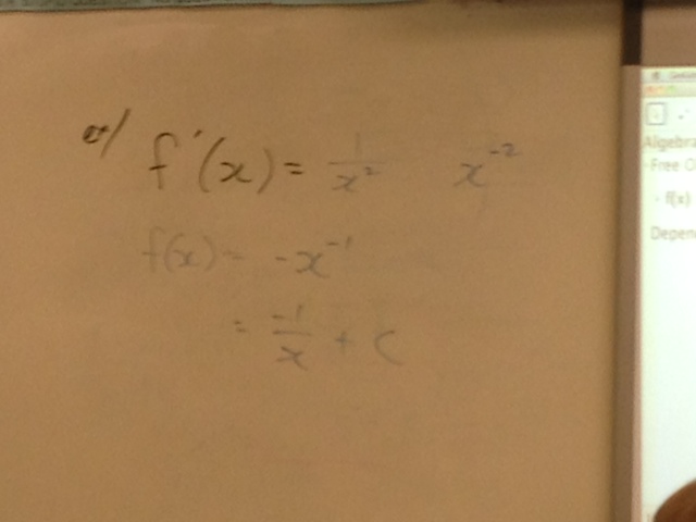
Do you follow what the example does? We know that when x is on the bottom of a fraction, that it can be written as being raised to a negative exponent. In this case,  . Using the knowledge Duncan showed so excellently in our first example, lets examine what our function should look like! To get a final value of , we will need a function which, when its exponent is multiplied out in front and then dropped by one, will end up as our desired derivative.
  fits well! Dropping down a negative one will make the derivative positive, and the power will descend to -2! But we know that a negative powers moves our x to the bottom of the fraction, leaving the -1 on top. Don't forget that there might be a constant c!
Confused? So was I! But then OB in his magnanimity decided to show the problem from another angle so that we might truly master its finer qualities. Let's use the natural log to get the same answer - just from a different angle!

We know that the derivative of  "This is the rendered form of the equation. You can not edit this directly. Right click will give you the option to save the image, and in most browsers you can drag the image onto your desktop or another program.") is
is  . In this case, the thing on the bottom of the fraction is an
  . Thus, we know that it must be what was initially natural log'd. Don't forget that constant c! Work backwards from the f(x) we found above if you're still confused - you'll see that taking its derivative works out. Oh wait... does it? When you bring the power out front, that function becomes
 +c "This is the rendered form of the equation. You can not edit this directly. Right click will give you the option to save the image, and in most browsers you can drag the image onto your desktop or another program.") . Its derivative wouldn't be what we're looking for, it would be
. Its derivative wouldn't be what we're looking for, it would be  , not
, not  like we wanted! Oh woe and sadness, whatever will we do? We could try dividing by 2...

No, that doesn't work. What if we squared it?

Well isn't that an interesting idea... What would that give us? It seems we would need the product and chain rules to fix this mess! This means *ln(x^2) "This is the rendered form of the equation. You can not edit this directly. Right click will give you the option to save the image, and in most browsers you can drag the image onto your desktop or another program.") . Thus, using the product rule we know that
. Thus, using the product rule we know that *ln(x^2){}'] "This is the rendered form of the equation. You can not edit this directly. Right click will give you the option to save the image, and in most browsers you can drag the image onto your desktop or another program.") . However, this is as far as we can go. There is only one antiderivative that can be found per equation, they are unique. MIT to the rescue again!
. However, this is as far as we can go. There is only one antiderivative that can be found per equation, they are unique. MIT to the rescue again!
*******************************************************************************
We have light homework tonight - IW 3 consists of only 8 problems! However, we do have a quiz next class covering IW's 1, 2 and 3, so if you haven't done 1 and 2 yet, get on them!
To wrap up class, we began an explanation of the Mean Value Theorem which we will have to finish for homework. This theorem, like this intermediate value theorem and extreme value theorem will be useful for reasons to be explained in the examination sheet we have for homework. While at the moment we aren't linking derivatives and integrals, we will be doing so in the future. When we get there, this theorem will be invaluable.
Let's look at the mean value theorem from a simplified perspective - say you're driving to Augusta from Camden, and you want to average a speed of 50mph for some reason only known to math problem creators. On the trip, at some point your instantaneous rate of speed must hit 50 mph. You may travel half the trip at 1 mph, but in the middle of your ride your speed must increase at an infinitely quick rate so that you can cover the other half at 99. Even when you jump from 1 to 99, your speed passes through 50mph at some point in time. If you're doing a more modest 40mph for half the trip, you must speed up so that your speedometer passes through 50 to reach 60 for the second half of the trip to average out at 50mph.

Here we see the secant line in red connecting the two endpoints of the segment we are studying - call it [a,b] - and the tan line in blue which is parallel to the secant when taken at some point c. OB seems interested - but why is that? As always, Wikipedia has all the answers to life. But why is this so? The exploration will show us.

Doesn't this remind you of something? Something that starts with an I? Something that starts with an Intermediate? Something that sounds like... shmitermediate shmalue shmeorem? Thats right! It does look like the Intermediate Value Theorem! You're so smart!

Looking at example 1 on the exploration quickly, we notice that there is indeed a point on the interval examined with has a tangent parallel to the secant line drawn between the two endpoints. It seems like the mean value theorem may well hold up. What does Gabe's head have to say about question 2?


Yes Gabe, I agree! It is interesting that its possible for there to be more than one point on a function which has a tangent parallel to a secant drawn between two endpoints of a section.
Alright everyone, make sure that you have the IW's finished tonight as well as the Mean Value Theorem sheet; rest up for the quiz tomorrow also, and don't let those mean values get you down. 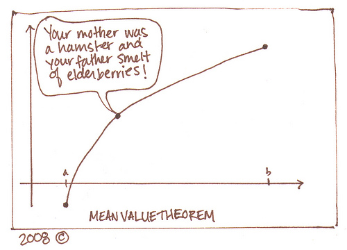
Wednesday, November 14, 2012
Scribe Post. 11/14
Today we began class by listening to a very intriguing piece about struggle and its connection to learning. We learned that "struggling is a chance to show that you have what it takes emotionally to overcome the problem, by having the strength to persist through that struggle" and that "academic success is not as much about whether a student is smart, academic success is about whether a student is willing to work and to struggle". As we listened to this, O'B was suggestively flaunting supercorrections as if there was a method to his madness. In case you're looking to get motivated, that piece by NPR can be found here. If that's not enough motivation, check out one of my personal favorites:
"When you want to breathe as bad as you want to succeed, then you'll be successful".
"Sleep is those people who are broke. I don't sleep"
It is hard work that makes a calculus student successful, and its hard work that makes math teachers smile

Next we talked a bit about supercorrections. If you didn't get them back today, you will get them back tomorrow. Also, prepare for the follow up test on Friday by using this blank copy of the test. Mr. O'B had the following words of wisdom for the following test problems to help us prepare for the follow-up:
#1: A derivative is a rate of change in a moment of time. It's the slope of the tangent line at any particular point
#2: Make sure you know the relationship between position, velocity, and acceleration
#3: If you want differentiability, you must have the same derivative from the left and right
#5: Make sure you're substituting in the Y value, not the X value!
#6: On the follow-up test, this question might be non-multiple choice. That means you can leave the answer in an form you'd like.
For the calculator side, don't forget about nDeriv and solver!
#7: Make sure you know derivatives of logs and inverse trig functions for the follow up
#8: Make sure you're comfortable with the limit definitions
#9: Sometimes you'll have to use the product rule in conjunction with the chain rule! Also know your log properties. They can be found here
#11: Know the derivatives of exponential functions.
#12: The follow up may ask a similar question but with inverse tangent or inverse cosecant
#13: The derivative finds you a slope of the tangent line at ANY point. You have to plug in the value of x to find the slope at a specific point.
#14: This is just simply asking for the derivative of cotangent evaluated at π/4
#15: Remember that with a limit definition, the slope of the tangent line on the top of the fraction divided by the slope of the tangent line on the bottom of the fraction will give you the limit value.
Mr. O'B then proceeded to tell us that the questions on the follow-up test will be completely random. He likened his method of choosing which questions to pick to the method by which George Bush's speeches are put together, as seen in this video: (skip to 1:24)

So, what this definition is basically saying is that the absolute max is the largest y value for a function, and the absolute min is the smallest y value for a function.
Let's put this into action by looking at the following functions on the following domains:

a)all reals
b) [0,2]
c) (0,2]
d) (0,2)
First let's look at the function with the domain of all reals:

So, this function has no absolute maximum, because it just keeps on going! However, it does have an absolute minimum. The absolute minimum is 0 when x=0.
Now let's look on the interval of [0,2]:

This has the same absolute minimum of 0 when x=0, but now there is a absolute maximum! Here the absolute maximum is 4 when x=2.
Now let's look at the interval of (0,2]:

Okay, so here again we have an absolute maximum of 4 when x=2. However, now that 0 isn't defined in our function, what is the smallest y value? What is the absolute minimum? Maybe it's .001? Or .00001? No no. You could go on and on, but there is always a smaller number you could stick in there, so there is actually NO absolute minimum for this function.
Now let's look at the interval of (0,2):

The same concept as we just discussed applies here. Since neither 0 nor 2 is defined in this function, what is the largest y value, and what is the smallest y value here? What are the absolute extrema's? Well in this case, there aren't actually any! When a function like this is on a completely open interval, there wont be any absolute extrema.
This brings us to the extreme value theorem which states that if a function is continuous on a closed interval [a,b], it will have an absolute max and an absolute min. Check out this applet that looks at the theorem. Look at these three graphs–they all are on the closed interval [a,b] and they all have global maximum and global minimum values:

Now it's time to look at relative extrema! To do this first, we looked at the definition on page 193. It is even more convoluted and confusing than the first definition we looked at! Hip hip hooray! Here it is:

So what this is basically saying is that if you look on a little open interval of a function, and you have a point that is the highest, or a point that is the lowest, you have local extrema! Following that logic, we can assert that if you look at all of the local extrema, you will find the global extrema as well! To get a more visual representation of this, we took a look at the figure on the same page:

So, as we can see here, this graph has local minimums, local maximums, absolute maximums, and absolute minimums. So, for example, if we're looking at the open interval of (a,e), the local maximum is indicated where x=c.
Notice anything about these local extrema? They occur in three places: where the derivative of the function is 0, where the derivative of the function is undefined, and at end points. Where f'(x) is equal to 0 or undefined are known as critical points. So, we can say that extrema only occur at critical points and end points. The derivative of the function is equal to 0 where you have a gradual change, such as at x=c. The derivative of the function is undefined at a cusp or corner such as where x=d. Critical points can be broken down even further into stationary points. Stationary points are where f'(x)=0. They are called this because that's where the function goes up, stops, then goes down, or goes up, stops, then keeps going up.
One thing to keep in mind is that just because you have critical points, DOESN'T mean you have extrema. Take this functions, for example:

You see, that at x=0, the derivative is equal to zero. Therefore, there is a critical point on this graph. However, this graph has no extrema! There are no values that are the lowest or the highest.
To finish up class, we took a look at two examples of the application of our newly found knowledge!
The first question asked us to find the extreme values of :
 on the closed interval of [-2,3] algebraically, then to confirm graphically.
So, here's what we have to do: We know that we'll find extrema where the derivative is 0, or undefined, or at end points. So, we need to solve for where the derivative is equal to zero, or undefined, and the endpoints, which are given to us as -2, and 3. With these values, we then need to plug back in to the original equation to see what values are the biggest or smallest to give us our extrema. Look at the following work below:

So, as you can see, when we find the derivative, it will never be equal to zero, so we must find where it will be undefined (where the denominator is equal to 0), and this occurs when x is zero. When we then plug in the critical points and end points, we can determine which is the smallest, and which is the biggest, which are our local extrema! We can now check this graphically to see if we're right! When we do that, we get the following graph:


"Sleep is those people who are broke. I don't sleep"
It is hard work that makes a calculus student successful, and its hard work that makes math teachers smile

Next we talked a bit about supercorrections. If you didn't get them back today, you will get them back tomorrow. Also, prepare for the follow up test on Friday by using this blank copy of the test. Mr. O'B had the following words of wisdom for the following test problems to help us prepare for the follow-up:
#1: A derivative is a rate of change in a moment of time. It's the slope of the tangent line at any particular point
#2: Make sure you know the relationship between position, velocity, and acceleration
#3: If you want differentiability, you must have the same derivative from the left and right
#5: Make sure you're substituting in the Y value, not the X value!
#6: On the follow-up test, this question might be non-multiple choice. That means you can leave the answer in an form you'd like.
For the calculator side, don't forget about nDeriv and solver!
#7: Make sure you know derivatives of logs and inverse trig functions for the follow up
#8: Make sure you're comfortable with the limit definitions
#9: Sometimes you'll have to use the product rule in conjunction with the chain rule! Also know your log properties. They can be found here
#11: Know the derivatives of exponential functions.
#12: The follow up may ask a similar question but with inverse tangent or inverse cosecant
#13: The derivative finds you a slope of the tangent line at ANY point. You have to plug in the value of x to find the slope at a specific point.
#14: This is just simply asking for the derivative of cotangent evaluated at π/4
#15: Remember that with a limit definition, the slope of the tangent line on the top of the fraction divided by the slope of the tangent line on the bottom of the fraction will give you the limit value.
Mr. O'B then proceeded to tell us that the questions on the follow-up test will be completely random. He likened his method of choosing which questions to pick to the method by which George Bush's speeches are put together, as seen in this video: (skip to 1:24)
Now we got down to business.
Our objective for today: Learn about absolute (global) extrema and relative (local) extrema.
To begin, we looked at the convoluted and confusing definition of absolute extrema values

So, what this definition is basically saying is that the absolute max is the largest y value for a function, and the absolute min is the smallest y value for a function.
a)all reals
b) [0,2]
c) (0,2]
d) (0,2)
First let's look at the function with the domain of all reals:

So, this function has no absolute maximum, because it just keeps on going! However, it does have an absolute minimum. The absolute minimum is 0 when x=0.
Now let's look on the interval of [0,2]:

This has the same absolute minimum of 0 when x=0, but now there is a absolute maximum! Here the absolute maximum is 4 when x=2.
Now let's look at the interval of (0,2]:

Okay, so here again we have an absolute maximum of 4 when x=2. However, now that 0 isn't defined in our function, what is the smallest y value? What is the absolute minimum? Maybe it's .001? Or .00001? No no. You could go on and on, but there is always a smaller number you could stick in there, so there is actually NO absolute minimum for this function.
Now let's look at the interval of (0,2):

The same concept as we just discussed applies here. Since neither 0 nor 2 is defined in this function, what is the largest y value, and what is the smallest y value here? What are the absolute extrema's? Well in this case, there aren't actually any! When a function like this is on a completely open interval, there wont be any absolute extrema.
This brings us to the extreme value theorem which states that if a function is continuous on a closed interval [a,b], it will have an absolute max and an absolute min. Check out this applet that looks at the theorem. Look at these three graphs–they all are on the closed interval [a,b] and they all have global maximum and global minimum values:

Now it's time to look at relative extrema! To do this first, we looked at the definition on page 193. It is even more convoluted and confusing than the first definition we looked at! Hip hip hooray! Here it is:

So what this is basically saying is that if you look on a little open interval of a function, and you have a point that is the highest, or a point that is the lowest, you have local extrema! Following that logic, we can assert that if you look at all of the local extrema, you will find the global extrema as well! To get a more visual representation of this, we took a look at the figure on the same page:

So, as we can see here, this graph has local minimums, local maximums, absolute maximums, and absolute minimums. So, for example, if we're looking at the open interval of (a,e), the local maximum is indicated where x=c.
Notice anything about these local extrema? They occur in three places: where the derivative of the function is 0, where the derivative of the function is undefined, and at end points. Where f'(x) is equal to 0 or undefined are known as critical points. So, we can say that extrema only occur at critical points and end points. The derivative of the function is equal to 0 where you have a gradual change, such as at x=c. The derivative of the function is undefined at a cusp or corner such as where x=d. Critical points can be broken down even further into stationary points. Stationary points are where f'(x)=0. They are called this because that's where the function goes up, stops, then goes down, or goes up, stops, then keeps going up.
One thing to keep in mind is that just because you have critical points, DOESN'T mean you have extrema. Take this functions, for example:

You see, that at x=0, the derivative is equal to zero. Therefore, there is a critical point on this graph. However, this graph has no extrema! There are no values that are the lowest or the highest.
To finish up class, we took a look at two examples of the application of our newly found knowledge!
The first question asked us to find the extreme values of :
So, here's what we have to do: We know that we'll find extrema where the derivative is 0, or undefined, or at end points. So, we need to solve for where the derivative is equal to zero, or undefined, and the endpoints, which are given to us as -2, and 3. With these values, we then need to plug back in to the original equation to see what values are the biggest or smallest to give us our extrema. Look at the following work below:

So, as you can see, when we find the derivative, it will never be equal to zero, so we must find where it will be undefined (where the denominator is equal to 0), and this occurs when x is zero. When we then plug in the critical points and end points, we can determine which is the smallest, and which is the biggest, which are our local extrema! We can now check this graphically to see if we're right! When we do that, we get the following graph:
Looks like we're spot on!
The next problem we looked at was to find the extreme values for the following function using a graphing calculator:
When you plug this into your calculator, it tricks you! It looks like there is both a global max and a global min. However, there is only a global minimum. This is because there are vertical asymptotes. However, the calculator doesn't show this, so it just looks like the function ends. Here is how you tackle this problem algebraically:

To make the derivative undefined, x has to be 2 or -2. To make the derivative zero, x must be 0. When you plug these values back into the original function, 2 and -2 make the function undefined (the vertical asymptote we already discussed), and 0 makes the function 1/2 which becomes our global minimum.
Update:
Thinking about all of these minimum's and maximum's, what does it all mean? Let's take a quick look at the connection between maximum's, minimum's, functions, first derivatives, and second derivatives.
So, think about the function x^2... We know what that looks like: a parabola opening upwards. So, we know that the function has a minimum at the very bottom of the curve. And at the bottom of the curve, the parabola flattens out for a second to give us local linearity, such that the slope at the very bottom is 0. That means that at the origin, when we look at our derivative, it will be zero. But what is the graph of the derivative doing before and after that? Well, let's think about to the left of the parabola. The slope is really really negative, and then as it gets closer and closer to zero it becomes less and less negative and begins to flatten out until it is zero, then to the right of the origin, the slope gets bigger and bigger and more positive. So, the derivative will start negative, pass through the origin (so it is equal to zero) then keep going up. It will be a line! In fact, it will be the line of 2x! Now what about the second derivative? The first derivative has a constant slope, which means that the second derivative will just be a line, the line of y=2 to be more exact! So, a graph with an absolute minimum has a derivative with a positive slope, and a second derivative that is a positive horizontal line. What about a graph with just an absolute maximum? Like -x^2. Think about everything we just talked about in reverse. The derivative will now have a negative slope, and the second derivative will be a negative horizontal line. The graph of -x^2 is known as concave down, and the graph of x^2 is known as concave up. These concavities can tell us a lot about the behavior of the first and second derivatives.
Subscribe to:
Comments (Atom)